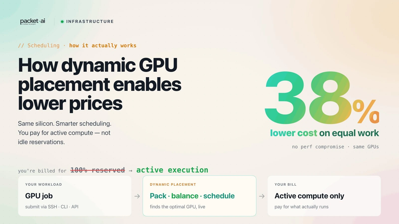
GPU pricing assumes 30% utilisation - you pay for the idle 70%. Here’s how dynamic placement achieves 5× better utilisation and why that drives packet.ai’s pricing.
Dynamic GPU placement on packet.ai schedules workloads based on real-time VRAM and compute usage - not static allocation. The result is GPU infrastructure that runs efficiently and charges you less for it.
Key takeaways
Most GPU cloud providers operate on a static allocation model: you rent a GPU, it is reserved for you, and you pay for it whether or not your workload is using 100% of it. A training job that uses 60 GB of a 80 GB GPU sits on reserved hardware with 20 GB of unused VRAM and variable SM utilisation depending on the training step.
From the cloud provider's perspective, that 20 GB of unused VRAM and the idle SM cycles are lost capacity. From your perspective, you are paying for hardware you are not fully utilising. Both problems have the same source: static allocation does not match supply to actual demand.
Dynamic placement changes this by making allocation decisions based on real-time resource profiles rather than worst-case reservations.
The packet.ai scheduler continuously monitors four dimensions of GPU resource usage across the fleet:
1. VRAM occupancy: How much of the GPU's memory is actively used vs allocated vs available. Not just the headline allocation - the live working set.
2. Memory bandwidth consumption: What fraction of the GPU's memory bandwidth is being consumed. An inference workload using 60 GB of VRAM but only 20% of memory bandwidth is a very different profile from a training workload using 60 GB with 90% bandwidth saturation.
3. SM (streaming multiprocessor) utilisation: What fraction of the GPU's compute units are active and executing kernels. High SM utilisation with low memory bandwidth indicates a compute-bound workload. Low SM with high bandwidth indicates a memory-bandwidth-bound workload.
4. PCIe and NVLink bandwidth: Data movement between host and device, and between GPUs. High PCIe bandwidth indicates active data loading (common in training); low indicates mostly in-GPU computation (common in steady-state inference).
These four dimensions define a "resource fingerprint" for each workload. The scheduler uses this to place workloads that are complementary on the same physical hardware - workloads whose resource fingerprints do not conflict.
The practical insight behind dynamic placement: most GPU workloads do not saturate all four resource dimensions simultaneously.
A steady-state LLM inference workload - serving tokens from a loaded model - typically uses 70-90% of VRAM, 40-60% of memory bandwidth (depending on batch size), and 30-50% of SM compute. PCIe bandwidth is low because the model is already in VRAM.
A batch preprocessing workload - tokenising and loading data for a training job - uses minimal VRAM, moderate PCIe bandwidth, and low SM utilisation.
These two workloads placed on the same GPU do not meaningfully conflict. The inference workload occupies VRAM the preprocessor does not need. The preprocessor uses PCIe bandwidth the inference workload is not consuming. SM contention is manageable because the preprocessor's GPU kernel footprint is small.
The scheduler identifies these complementary profiles and places them together. The result: higher fleet utilisation without meaningful performance degradation for either workload.
The scheduler does not co-locate workloads indiscriminately. Co-location is rejected when:
The latency-sensitivity flag is set automatically for workloads in Dedicated tier. Dynamic tier workloads are assumed to be latency-tolerant (batch inference, training, fine-tuning, experiments).
A common misconception: Dynamic tier uses lower-quality or older hardware than Dedicated. This is not the case.
Both tiers run on the same physical GPU fleet. An A100 80GB in Dynamic capacity is the same A100 80GB as in Dedicated capacity - same silicon, same VRAM, same memory bandwidth, same compute. What differs is the scheduling model.
Dedicated capacity pins the GPU to your workload for the duration of your session. The scheduler will not place another workload on that hardware while your job is running. You get 100% of the GPU's resources exclusively.
Dynamic capacity allows the scheduler to co-locate complementary workloads on the same hardware. Your workload gets a resource allocation that is guaranteed not to conflict with co-located workloads - but the guarantee is at the resource level, not the hardware level.
The price difference between Dynamic and Dedicated reflects this scheduling model difference. Dynamic is cheaper because the fleet runs at higher utilisation, reducing the per-hour cost of the underlying hardware.
Because the scheduler only co-locates non-conflicting workloads, performance on Dynamic capacity is typically within 2-5% of Dedicated for throughput-oriented workloads (training loss curves, tokens/second for batch inference, image generation throughput).
Where Dynamic and Dedicated diverge is tail latency under load. Co-located workloads create minor SM scheduling contention at the GPU hardware level - not visible in average throughput but present in p99 and p999 latency distributions. For production inference APIs with strict TTFT (time to first token) SLAs, Dedicated is the right choice. For training and batch workloads, Dynamic capacity is effectively equivalent in practice.
Dynamic placement keeps the packet.ai fleet running at above 85% GPU utilisation during peak hours. This matters to you for two reasons:
Pricing: Higher fleet utilisation means lower per-hour cost of running the infrastructure. That cost reduction flows through to Dynamic tier pricing. The gap between Dynamic and Dedicated pricing reflects the utilisation efficiency the scheduler enables.
Availability: A fleet running at 85% utilisation through scheduling efficiency has more capacity headroom than a fleet running at 85% through raw demand. The scheduler can compress existing workloads to free capacity for new ones, rather than simply reporting "no capacity available".
Static allocation clouds typically run at 30-60% utilisation before capacity adjustments. The difference between 40% and 85% fleet utilisation represents a significant infrastructure cost difference that eventually shows up in pricing tiers.
Same models. Same API. Fraction of the cost. Start free — no credit card required.
Start Building →